 So this is my first real post here! After studying deep learning for a while I wanted to go back to the basics and explain to myself (and others) in a straightforward and comprehensive manner how I understood the mechanisms underlying neural nets when learning about them. I’m doing this in part since I wanted to get this blog started at some point (lol) but also because it’s fun to go back and dive into the basics of what inspired most cutting edge systems today. When I started to grasp how these worked it really was an aha moment for me and I hope you get that moment too, especially if you’re just getting started with deep learning coming from linear models, this is where it gets interesting. The mechanisms are pretty complex to make sense of the first time and from afar it’s truly amazing to see that these things even work in the first place. I hope you find this interesting and helpful! A lot of the following is from my notes so please do point out any mistakes / inaccuracies or drop a question if you have one to darius.foodei@gmail.com . Btw I apologize in advance if Latex fails to render correctly sometimes the library I’m using is a bit buggy and I’m still figuring out how to fix it.
Introduction
So let’s dive in! If you’ve studied linear models for regression and classification you’ve probably seen until now that these models are simple and quite effective in many cases. You’ve also probably seen that transforming the input non linearly using feature expansion and kernel methods gives you more flexibility to separate classes since it allows you to distinguish more complex patterns and more effectively parse the data. Nevertheless, the transformations were all manual until now. What I mean by this is that they were done independently of the model so you had no guarantee that your choices were the best or the most optimal. Neural networks represent an advanced evolution in computational models, closely mirroring the brain’s ability to discern patterns and classify information. These networks autonomously detect and learn from patterns in data, offering insights into complex problems in a way that’s reminiscent of human cognitive processes.
Basic example, the polynomial curve fitting
You’ve probably seen that you can use polynomial feature expansion followed by applying a linear model to the expanded features. In this case the feature expansion was manually defined, independently of the linear model. We want to be able to learn the feature expansion and the linear model jointly.
We need a feature expansion that depends on parameters so that we can train those parameters with the parameters of our classifier.
To achieve this, we can define a parametric feature expansion strategy that introduces non linearity in the process. We can use a nonlinear function $f : \mathbb{R} \to \mathbb{R}$ and define the following :
$$ \mathbf{a}^{(1)} = \mathbf{W_{(1)}^{T}} \begin{bmatrix} 1 \\ \mathbf{x} \end{bmatrix} = \begin{bmatrix} W_{(1)}^{(1,0)} + W_{(1)}^{(1,1)}x \\ W_{(1)}^{(2,0)} + W_{(1)}^{(2,1)}x \\ \vdots \\ W_{(1)}^{(M,0)} + W_{(1)}^{(M,1)}x \\ \end{bmatrix} = \begin{bmatrix} a_{(1)}^{(1)} \\ a_{(1)}^{(2)} \\ \vdots \\ a_{(1)}^{(M)} \\ \end{bmatrix} $$
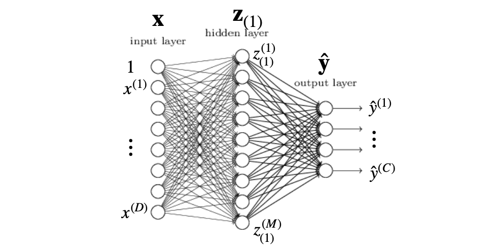
Then, our parametric feature expansion process can be expressed as (figure 1) :
$$ \mathbf{x} \rightarrow \begin{bmatrix} f(a_{(1)}^{(1)}) \\ f(a_{(1)}^{(2)}) \\ \vdots \\ f(a_{(1)}^{(M)}) \end{bmatrix} = f \left(\mathbf{W_{(1)}}^{T}\begin{bmatrix}1 \\ \mathbf{x}\end{bmatrix}\right)=z_{(1)} $$
where the final notation applies the non-linear function $f$ in an element wise manner to the M-dimensional vector output by the linear mapping. In the context of artificial neural networks the function $f$ would be referred to as the activation function.
The M-dimensional vector (figure 1) is commonly referred to as a hidden representation (or a hidden layer) each M element is a hidden unit or “neuron”. It’s important to note that the $(1)$ subscript denotes the layer number.
Typical activation functions
- Sigmoid : $f(a) = \frac{1}{1+exp(-a)}$
- Hyperbolic tangent : $f(a) = tanh(a)$
- Rectified Linear Unit (ReLU): $f(a) = \begin{cases} a, & \text{if } a > 0 \ 0, & \text{otherwise} \end{cases} = \max(a, 0)$
Complete model
We can then perform prediction by applying a second linear model to the hidden representation which gives:
$$ \hat{y} = \mathbf{w_{(2)}}^{T} \mathbf{z_{(1)}} = \mathbf{w_{(2)}}^{T} f \left( \mathbf{W_{(1)}}^{T} \begin{bmatrix} 1 \\ \mathbf{x} \end{bmatrix} \right) = \mathbf{w_{(2)}}^{T} \begin{bmatrix} f(a_{(1)}^{(1)}) \\ f(a_{(1)}^{(2)}) \\ \vdots \\ f(a_{(1)}^{(M)}) \end{bmatrix} = \sum_{j=1}^{M} w_{(2)}^{(j)} f \left( W_{(1)}^{(j,0)} + W_{(1)}^{(j,1)} x \right) $$
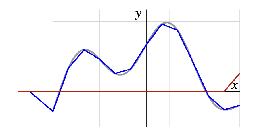
We can approximate any continuous function with a linear combination of translated/scaled ReLU functions $f(…)$ :
$$ \hat{y} = w_{(2)}^{(1)} f \left( W_{(1)}^{(1,0)} + W_{(1)}^{(1,1)} x \right) + w_{(2)}^{(2)} f \left( W_{(1)}^{(2,0)} + W_{(1)}^{(2,1)} x \right) + w_{(2)}^{(3)} f \left( W_{(1)}^{(3,0)} + W_{(1)}^{(3,1)} x \right) + \ldots $$

The image above shows a piecewise linear function which approximates a continuous function using a combination of scaled and translated ReLU functions. Recall that the ReLU function is defined as $f(x) = \max(0, x)$, which means it outputs zero for any negative input and outputs the input itself for any positive input.
-
Piecewise Linear Nature: Each segment corresponds to a part of the function where the ReLU is active (i.e., the input to the ReLU is positive).
-
Points of Change (Kinks): Wherever there’s a ‘kink’ or change in the direction of the line, it corresponds to a point where a particular ReLU function transitions from inactive to active (or vice versa). The kinks are the points where the input to a ReLU function is zero.
-
Modeling Nonlinear Functions: Even though each individual ReLU function is linear (for positive values), combining them allows the model to approximate a nonlinear function to capture complex patterns in data.
The weights and biases determine the shape and position of each linear segment, and their proper adjustment during the training process enables the network to closely approximate a target function.
Multiple input dimensions
Handling $(D > 1)$ input dimensions makes very little difference in the model formulation. From the 1D input formulation :
$$ \hat{y} = \mathbf{W_{(2)}}^{T} f \left(\mathbf{W}^{T}_{(1)} \begin{bmatrix} 1 \\ \mathbf{x} \end{bmatrix} \right) $$
we simply write the $D$-dimensional case as :
$$ \hat{y} = \mathbf{W_{(2)}}^{T} f \left( \mathbf{W}^{T}_{(1)} \mathbf{x} \right) $$
where $\mathbf{x} \in \mathbb{R}^{D+1}$ to account for the bias, and $\mathbf{W}_{(1)}$ is of dimension $(D + 1) \times M$ instead of $2 \times M$.
Multiple output dimensions
To handle $C \geq 1$ output dimensions, we can proceed as in the case of linear models. We simply need to replace the vector of parameters $W_{(2)}$ with a matrix of parameters $W_{(2)} \in \mathbb{R}^{M \times C}$
The prediction can then be written as :
$$\hat{y} = W^{T_{(2)}} f \left( W^{T}_{(1)} x \right)$$
where $\hat{y} \in \mathbb{R}^C$ is now a vector of dimension $C$ (multiple output dimensions).

We say the layers are fully connected since we use a matrix-vector product for each layer.
The multilayer perceptron model
With a single layer, one can already model complicated functions but why stop here. We can add hundreds if not thousands of hidden layers to model basically anything. Generally, more layers can model more complex patterns but may lead to overfitting and require more data and training time so it’s important to keep this in mind when designing and testing your network.
Each hidden layer of the perceptron takes as input the output of the previous layer. For the first hidden layer i.e. the input layer, we still have :
$$z_{(1)} = f \left( W_{(1)}^T x \right)$$
For any subsequent layer $( l )$, we have :
$$z_{(l)} = f \left( W_{(l)}^T z_{(l-1)} \right)$$
where you can see the previous layer being used as input. Finally, for a network of ( L ) layers, we compute the output as :
$$\hat{y} = W_{(L)}^T z_{(L-1)}$$
The process of going from the input to the output is called the forward pass of the network.
If we wanted to write the prediction of the network as a single equation, it would look like :
$$\hat{y} = W_{(L)}^T f \left( W_{(L-1)}^T f \left( W_{(L-2)}^T f \left( \cdots f \left( W_{(1)}^T x \right) \cdots \right) \right) \right)$$
This is not very convenient, and it is easier to simply think of $\hat{y}$ as a function of all parameters :
$$\hat{y} = \hat{y}(W)$$
where $W = { W_{(l)} }$ encompasses all the parameters from every layer.
Training a MLP
With a given set of N training samples $(x_{i}, y_{i})$ , we now want to find the best set of parameters $W^{*}$. As usual we do this by minimising the empirical risk w.r.t. all the parameters $W$.
Because a MLP stacks multiple layers which each has a nonlinear activation function, the problem does not have a closed form convex solution. Learning is therefore done by gradient descent. While the gradient might seem like hell to compute, it can in fact be computed in a pretty neat way thanks to back propagation.
Since the empirical risk is an average over the training samples, it’s gradient will also be an average of gradients. We can focus on a single loss term :
$$R({W_{(l)}}) = \frac{1}{N} \sum_{i=1}^{N} \ell(\hat{y_i}, y_i) = \frac{1}{N} \sum_{i=1}^{N} \ell_i$$
For the $k^{th}$ dimension of the output of any layer $l$, let us define :
$$a_{(l)}^{(k)} = \sum_j W_{(l)}^{(k,j)} z_{(l-1)}^{(j)}$$
which denotes the dot product between the $k^{th}$ column of $W_{(l)}$ and $z_{(l-1)}$.
What we aim to compute is the derivative of the loss function $\ell_i$ w.r.t. any parameter $W^{(k,j)}_{(l)}$
Following the chain rule, we can write such a derivative as :
$$ \frac{\partial \ell_i}{\partial W_{(l)}^{(k,j)}} = \frac{\partial \ell_i}{\partial a_{(l)}^{(k)}} \frac{\partial a_{(l)}^{(k)}}{\partial W_{(l)}^{(k,j)}} = \frac{\partial \ell_i}{\partial a_{(l)}^{(k)}} z_{(l-1)}^{(j)} $$
Furthermore, let us define :
$$ \delta_{(l)}^{(k)} = \frac{\partial \ell_i}{\partial a_{(l)}^{(k)}} $$
which directly encodes the first term of the derivative. So now we can rewrite the derivative :
$$ \frac{\partial \ell_i}{\partial W_{(l)}^{(k,j)}} = \delta_{(l)}^{(k)} z_{(l-1)}^{(j)}$$
Because the hidden values $z_{(l-1)}^{(j)}$ are computed in the forward pass, we only need to compute the ${\delta^{(k)}_{(l)}}$ to obtain the derivative of the loss w.r.t. any parameter.
For the last layer (Layer $L$), we have (assuming no final activation) :
$$ a^{(k)}_{(L)} = \hat{y}^{(k)} $$
This means that, for the last layer, $\delta^{(k)}_{(L)}$ can be computed explicitly as the partial derivative of the loss function w.r.t. the network’s output.
E.g., for the square loss, we have :
$$ \delta_{(L)}^{(k)} = 2(\hat{y_{i}}^{(k)} - y_{i}^{(k)}) $$
For the other layers ($l < L$), it can be shown that $\delta^{(k)}_{(l)}$ can be computed from :
- the ${\delta^{(j)}_{(l+1)}}$ (from the subsequent layer $l + 1$)
- the derivative of the activation function w.r.t. its input
- the parameters $W_{(l+1)}$ (of the subsequent layer $l + 1$)
In other words, given $\delta_{(l+1)}$, one can compute $\delta_{(l)}$ Because we can explicitly compute $\delta_{(L)}$ for the last layer, we can in turn compute any $\delta_{(l)}$. Then, this gives us a way to compute the gradient :
$$ \frac{\partial \ell_i}{\partial W_{(k,j)}^{(l)}} = \delta_{(l)}^{(k)} z_{(l-1)}^{(j)} $$
at any layer, starting from the last one. Which brings us to the big daddy of neural nets.
The back propagation algorithm
I won’t go into too much details as it can quickly get messy but the general idea is the following :
- Propagate $x_i$ (our data) forward through the network
- Compute $\delta_{(L)}$ (last layer) depending on the loss
- Propagate $\delta_{(L)}$ backward to obtain each $\delta_{(l)}$ (hidden layers)
- At each layer, compute the partial derivatives
$$ \frac{\partial \ell_i}{\partial W_{(k,j)}^{(l)}} = \delta_{(l)}^{(k)} z_{(l-1)}^{(j)} $$
where $z_{(l-1)}$ has been computed during the forward pass.
This is the part where all the different indexes were driving me crazy so as a reminder :
- $l$ : Refers to the $l$-th layer in the network. $l=1$ refers to the input layer and $l=L$ refers to the output layer.
- $k$ : Refers to the $k$-th neuron in the $l$-th layer.
- $j$ : Refers to the $j$-th neuron in the $(l-1)$-th layer. This neuron’s activation is being used in the calculation of the gradient for the 𝑘-th neuron’s weights in the 𝑙-th layer.
- $i$ : Refers to the 𝑖-th data point or input sample from the training dataset.
Moving on, once the gradient is computed, the update at iteration $k$ is performed as
$$ W_k \leftarrow W_{k-1} - \eta \nabla_{W} R(W_{k-1}) $$
where $W$ encompasses the parameters of all layers. This should look familiar if you’ve seen how linear models are trained already.
You can also think of this as updating the parameters in each layer $l$ as :
$$ W_{(l),k} \leftarrow W_{(l),k-1} - \eta \nabla_{W_{(l)}} R(W_{k-1}) $$
where $W_{(l),k}$ represents the parameters of layer $l$ at iteration $k$ during gradient descent.
Because the gradient of an average is the average of the gradients, we can also write a standard gradient update as :
$$ W_k \leftarrow W_{k-1} - \eta \frac{1}{N} \sum_{i=1}^{N} \nabla_{W} \ell_i(W_{k-1}) $$
This means that, for each gradient descent iteration, one needs to perform a forward pass and a backward pass through the network for all the training samples
- As you can probably guess this becomes expensive for large training sets…
Stochastic Gradient Descent
The solution to this is stochastic gradient descent which updates the parameters $W$ based on the gradient of a single sample in each iteration :
$$ W_k \leftarrow W_{k-1} - \eta \nabla{l_{i(k)}} (W_{k-1}) $$
At each iteration we use the gradient of a single loss term. The index of the sample depends on the iteration number k.
In practice, one iterates over the training samples, either in a fixed order or randomly.
SGD with mini-batches
The gradient obtained by a single sample might be a poor approximation of the true, complete gradient. E.g., an individual sample might benefit from the increase of one specific parameter, whereas most of the other samples would benefit from a decrease of this parameter.
To obtain a more reliable gradient estimate, one typically uses mini-batches of $B$ samples.
The parameters are then updated as follows :
$$ W_k \leftarrow W_{k-1} - \eta \sum_{b=1}^{B} \nabla \ell_{i(b,k)}(W_{k-1}) $$
The index of the samples used for the update now depends on the iteration number $k$ AND the index $b$ of the samples in the mini-batch.
SGD Extensions
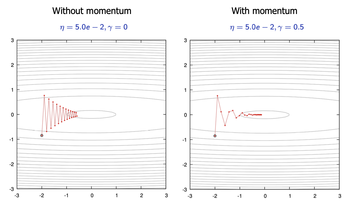
To improve the convergence speed and performance of SGD, several extensions have been developed. One of the most significant of these is momentum: The idea is that you add inertia to the parameter updates :
$$ \nu \leftarrow \gamma \nu + \eta \nabla R(W) $$
$$ W \leftarrow W - \nu $$
With $\gamma > 0$, momentum then
- accelerates if the gradient does not change too much.
- dampens the oscillations in narrow valleys.

What about classification?
So far, we have focused on the case where the prediction is taken directly as the output of a linear model applied to the last hidden representation, i.e.,
$$ \hat{y} = W_{(L)}^T z_{(L-1)} $$
While this is fine for a regression task, it is not ideal for a classification one, where we would like each $\hat{y}^{(k)}$ to represent the probability (score) for class $k$.
This can be achieved via the softmax function (as in multi-class logistic regression) :
$$ \hat{y}^{(k)} = \frac{\exp(W_{(L)}^{(k)T} z_{(L-1)})}{\sum_{j=1}^{C} \exp(W_{(L)}^{(j)T} z_{(L-1)})} $$
where $W_{(L)}^{(j)}$ indicates the $j^{th}$ column of $W_{(L)}$. In this case, the empirical risk is typically defined as the cross-entropy :
$$ R(W) = -\frac{1}{N} \sum_{i=1}^{N} \sum_{k=1}^{C} y_i^{(k)} \ln \hat{y}_i^{(k)} $$
Back propagation then requires computing the derivative of the cross-entropy w.r.t. each $\hat{y}^{(k)}$ and the derivative of the softmax function w.r.t. each $W_{(j,k)}^{(L)}$
- Note that this is similar to the derivatives computed for multi-class logistic regression.
I could detail this but the idea is very similar and there are a bunch of examples online.
If you got until here thanks for taking the time! I hope this gave you a better idea of how all these different elements work together mathematically. Personally, it really took me a moment to wrap my head around these concepts and going step by step like this helped me a lot to visualize. I hope to post asap about more interesting and advanced subjects like RNNs and CNNs once I finish writing about them so come back soon!
References
- CS233 - “Introduction to Machine Learning” course at EPFL - Fua, Salzmann
- Deep Learning - Goodfellow, Bengio, Courville
- CS231n - “Convolutional Neural Networks for Visual Recognition” course at Stanford
- CS229 - “Machine Learning” course at Stanford